Traffic Sign Recognition with Tensorflow
Introduction
In this project, I used a convolutional neural network (CNN) to classify traffic signs. I trained and validated a model so it can classify traffic sign images using the German Traffic Sign Dataset. After the model is trained, I tried out the model on images of traffic signs that I took with my smartphone camera.
My final model results are:
- Training set accuracy of 97.5%
- Validation set accuracy of 98.5%
- Test set accuracy of 97.2%
- New Test set accuracy of 100% (6 new images taken by me)
Here is the project code. Please note that I used only the CPU of my laptop to train the network.
The steps of this project are the following:
- Load the data set
- Explore, summarize and visualize the data set
- Design, train and test a model architecture
- Use the model to make predictions on new images
- Analyze the softmax probabilities of the new images
- Summarize the results with a written report
Data Set Summary & Exploration
1. Basic summary of the data set
I used the Pandas library to calculate summary statistics of the traffic signs data set:
- The size of original training set is 34799
- The size of the validation set is 4410
- The size of test set is 12630
- The shape of a traffic sign image is 32x32x3 represented as integer values (0-255) in the RGB color space
- The number of unique classes/labels in the data set is 43
We have to work with images with a resolution of 32x32x3 representing 43 type of different German traffic signs.
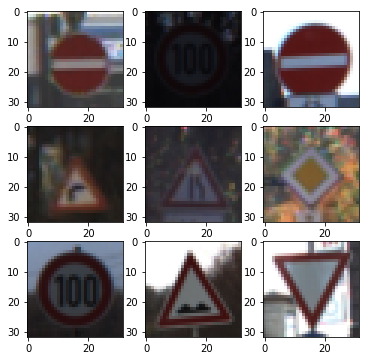
2. Exploratory visualization of the dataset
Here is an exploratory visualization of the data set. It is a bar chart showing how many samples we have for each class.
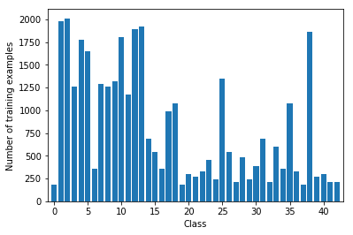
We can notice that the distribution is not balanced. We have some classes with less than 300 examples and other well represented with more than 1000 examples. We can analyze now the validation dataset distribution:

The distributions are very similar. Even if it would be wise to balance the dataset, in this case, I am not sure it would be very useful. In fact, some traffic signs (for example the 20km/h speed limit) could occur less frequently than others (the stop sign for example). For this reason I decided to not balance the dataset.
Class 0: Speed limit (20km/h)                                180 samples
Class 1: Speed limit (30km/h)                                1980 samples
Class 2: Speed limit (50km/h)                                2010 samples
Class 3: Speed limit (60km/h)                                1260 samples
Class 4: Speed limit (70km/h)                                1770 samples
Class 5: Speed limit (80km/h)                                1650 samples
Class 6: End of speed limit (80km/h)                         360 samples
Class 7: Speed limit (100km/h)                               1290 samples
Class 8: Speed limit (120km/h)                               1260 samples
Class 9: No passing                                          1320 samples
Class 10: No passing for vehicles over 3.5 metric tons        1800 samples
Class 11: Right-of-way at the next intersection               1170 samples
Class 12: Priority road                                       1890 samples
Class 13: Yield                                               1920 samples
Class 14: Stop                                                690 samples
Class 15: No vehicles                                         540 samples
Class 16: Vehicles over 3.5 metric tons prohibited            360 samples
Class 17: No entry                                            990 samples
Class 18: General caution                                     1080 samples
Class 19: Dangerous curve to the left                         180 samples
Class 20: Dangerous curve to the right                        300 samples
Class 21: Double curve                                        270 samples
Class 22: Bumpy road                                          330 samples
Class 23: Slippery road                                       450 samples
Class 24: Road narrows on the right                           240 samples
Class 25: Road work                                           1350 samples
Class 26: Traffic signals                                     540 samples
Class 27: Pedestrians                                         210 samples
Class 28: Children crossing                                   480 samples
Class 29: Bicycles crossing                                   240 samples
Class 30: Beware of ice/snow                                  390 samples
Class 31: Wild animals crossing                               690 samples
Class 32: End of all speed and passing limits                 210 samples
Class 33: Turn right ahead                                    599 samples
Class 34: Turn left ahead                                     360 samples
Class 35: Ahead only                                          1080 samples
Class 36: Go straight or right                                330 samples
Class 37: Go straight or left                                 180 samples
Class 38: Keep right                                          1860 samples
Class 39: Keep left                                           270 samples
Class 40: Roundabout mandatory                                300 samples
Class 41: End of no passing                                   210 samples
Class 42: End of no passing by vehicles over 3.5 metric tons  210 samples
Design and Test a Model Architecture
1. Pre-processing
This phase is crucial to improving the performance of the model. First of all, I decided to convert the RGB image into grayscale color. This allows to reduce the numbers of channels in the input of the network without decreasing the performance. In fact, as Pierre Sermanet and Yann LeCun mentioned in their paper “Traffic Sign Recognition with Multi-Scale Convolutional Networks”, using color channels did not seem to improve the classification accuracy. Also, to help the training phase, I normalized each image to have a range from 0 to 1 and translated to get zero mean. I also applied the Contrast Limited Adaptive Histogram Equalization (CLAHE), an algorithm for local contrast enhancement, which uses histograms computed over different tile regions of the image. Local details can, therefore, be enhanced even in areas that are darker or lighter than most of the image. This should help the feature exaction.
Here the function I used to pre-process each image in the dataset:
def pre_processing_single_img (img):

    img_y = cv2.cvtColor(img, (cv2.COLOR_BGR2YUV))[:,:,0]
    img_y = (img_y / 255.).astype(np.float32)
    img_y = (exposure.equalize_adapthist(img_y,) - 0.5)
    img_y = img_y.reshape(img_y.shape + (1,))

    return img_y
Steps:
Convert the image to YUV and extract Y Channel that correspond to the grayscale image:
img_y = cv2.cvtColor(img, (cv2.COLOR_BGR2YUV))[:,:,0]Y stands for the luma component (the brightness) and U and V are the chrominance (color) components.Normalize the image to have a range from 0 to 1:
` img_y = (img_y / 255.).astype(np.float32) `Contrast Limited Adaptive Histogram Equalization (see here for more information) and translate the result to have mean zero:
img_y = (exposure.equalize_adapthist(img_y,) - 0.5)Finally reshape the image from (32x32) to (32x32x1), the format required by tensorflow:
img_y = img_y.reshape(img_y.shape + (1,))
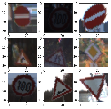
Here is an example of a traffic sign image before and after the processing:
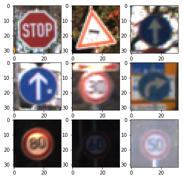
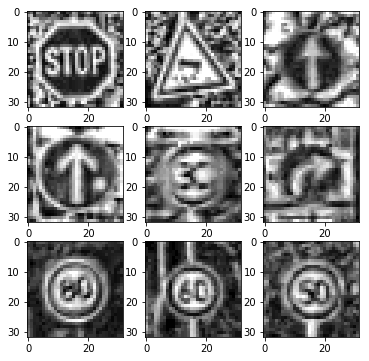
Initially, I used .exposure.adjust_log, that it is quite fast but finally I decided to use exposure.equalize_adapthist, that gives a better accuracy.
2. Augmentation
To add more data to the data set, I created two new datasets starting from the original training dataset, composed by 34799 examples. In this way, I obtain 34799x3 = 104397 samples in the training dataset.
Keras ImageDataGenerator
I used the Keras function ImageDataGenerator to generate new images with the following settings:
datagen = ImageDataGenerator(
        rotation_range=17,
        width_shift_range=0.1,
        height_shift_range=0.1,
        shear_range=0.3,
        zoom_range=0.15,
        horizontal_flip=False,
        dim_ordering='tf',
        fill_mode='nearest')

 # configure batch size and retrieve one batch of images

for X_batch, y_batch in datagen.flow(X_train, y_train, batch_size=X_train.shape[0], shuffle=False):
    print(X_batch.shape)
    X_train_aug = X_batch.astype('uint8')
    y_train_aug = y_batch
    break
To each picture in the training dataset, a rotation, a translation, a zoom and a shear transformation is applied.
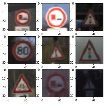
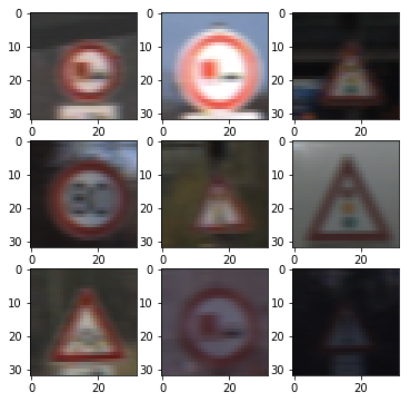
Here is an example of an original image and an augmented image:
Motion Blur
Motion blur is the apparent streaking of rapidly moving objects in a still image. I thought it is a good idea add motion blur to the image since they are taken from a camera placed on a moving car.
3. Final model architecture
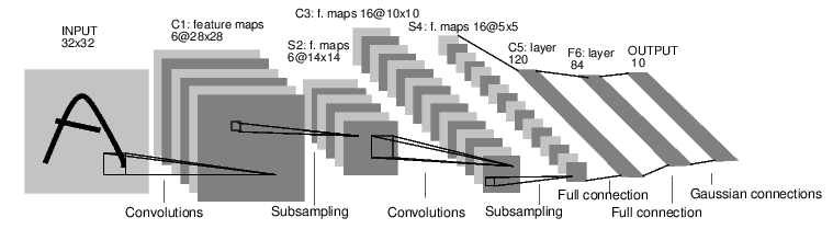
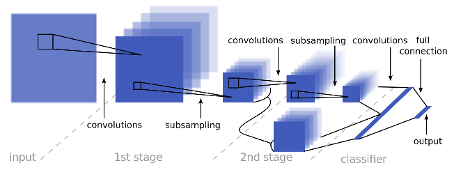
I started from the LeNet network and I modified it using the multi-scale features took inspiration from the model presented in Pierre Sermanet and Yann LeCun paper. Finally, I increased the number of filters used in the first two convolutions. We have in total 3 layers: 2 convolutional layers for feature extraction and one fully connected layer used. Note that my network has one convolutional layer less than the [Pierre Sermanet and Yann LeCun (http://yann.lecun.com/exdb/publis/pdf/sermanet-ijcnn-11.pdf) version.
| Layer | Description |
|---|---|
| Input | 32x32x1 Grayscale image |
| Convolution 3x3 | 1x1 stride, same padding, outputs 28x28x12 |
| RELU | |
| Max pooling | 2x2 stride, outputs 14x14x12 |
| Dropout (a) | 0.7 |
| Convolution 3x3 | 1x1 stride, same padding, outputs 10x10x24 |
| RELU | |
| Max pooling | 2x2 stride, output = 5x5x24. |
| Dropout (b) | 0.6 |
| Fully connected | max_pool(a) + (b) flattend. input = 1188. Output = 320 |
| Dropout (c) | 0.5 |
| Fully connected | Input = 320. Output = n_classes |
| Softmax |
To train the model I used 20 epochs with a batch size of 128, the AdamOptimizer(see paper here) with a learning rate of 0.001. The training phase is quite slow using only CPU, that’s why I used only 20 epochs.
My final model results were:
- Training set accuracy of 97.5%
- Validation set accuracy of 98.5%
- Test set accuracy of 97.2%
First attempt: validation accuracy 91.5%
Initially, I started with the LeNet architecture, a convolutional network designed for handwritten and machine-printed character recognition.
I used the the following preprocess pipeline:
- Convert in YUV, keep the Y
- Adjust the exposure
- Normalization
Parameters:
- EPOCHS = 10
- BATCH_SIZE = 128
- Learning rate = 0.001
Number of training examples = 34799
Number of validation examples = 4410
Number of testing examples = 12630
At each step, I will mention only the changes I adopted to improve the accuracy.
Second attempt: validation accuracy 93.1%
I added Dropout after each layer of the network LeNet:
1) 0.9 (after C1)
2) 0.7 (after C3)
3) 0.6 (after C5)
4) 0.5 (after F6)
Third attempt: validation accuracy 93.3%
I changed the network using multi-scale features as suggested in the paper Traffic Sign Recognition with Multi-Scale Convolutional Networks and use only one fully connected layer at the end of the network.
Fourth attempt: validation accuracy 94.6%
I augmented the training set using the Keras function ImageDataGenerator. In this way, I double the training set.
Number of training examples = 34799x2 = 69598
Number of validation examples = 4410
I Used Dropout with the follow probability (referred this table):
a) 0.8
b) 0.7
c) 0.6
Fifth attempt: validation accuracy 96.1%
Since the training accuracy was not very high, I decided to increase the number of filters in the first two convolutional layers.
First layer: from 6 to 12 filters.
Second layer: from 16 to 24 filters.
Final attempt: validation accuracy 98.5%
I augmented the data adding the motion blur to each sample of the training data. Hence, I triplicate the number of samples in the training set. In addition, I added the L2 regularization and I used the function equalize_adapthist instead of .exposure.adjust_log during the image preprocessing.
Performance on the test set
Finally I evaluated the performance of my model with the test set.
Accuracy
The accuracy was equal to 97.2%.
Precision
The Precision was equal to 96.6%
The precision is the ratio tp / (tp + fp) where tp is the number of true positives and fp the number of false positives. The precision is intuitively the ability of the classifier not to label as positive a sample that is negative.
Recall
The recall was equal to 97.2% The recall is the ratio tp / (tp + fn) where tp is the number of true positives and fn the number of false negatives. The recall is intuitively the ability of the classifier to find all the positive samples.
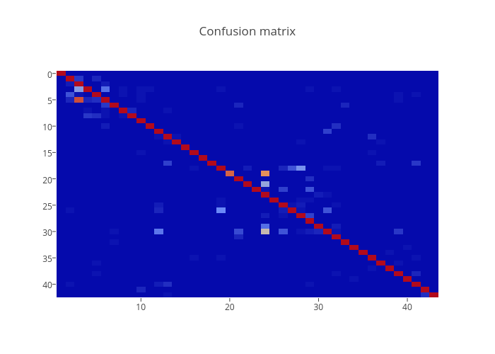
Confusion matrix
Let’s analyze the confusion matrix:
You can click on the picture to interact with the map.
We can notice that:
- 28/60 samples of to the class 19 (Dangerous curve to the left) are misclassified as samples belonging to the class 23 (Slippery road). This can be explained by the fact that the class number 19 is underrepresented in the training set: it has only 180 samples.
- 34/630 samples of to the class 5 (Speed limit 80km/h) are misclassified as samples belonging to the class 2 (Speed limit 50km/h).
- The model is not very good to classify the class number 30 (Beware of ice/snow), it classified samples in a wrong way 61 times.
- The model produces 80 false positives for the class 23.
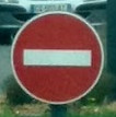
Test a Model on New Images
Here are five traffic signs from some pictures I took in France with my smartphone:


Here are the results of the prediction:
- the first image is the test image
- the second one is a random picture of the same class of the prediction
- the third one is a plot showing the top five soft max probabilities
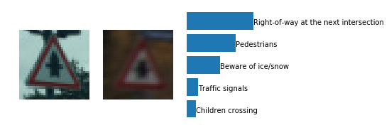
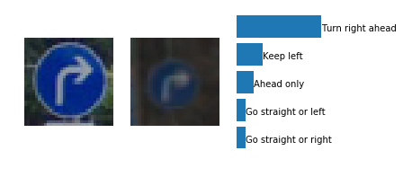
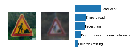
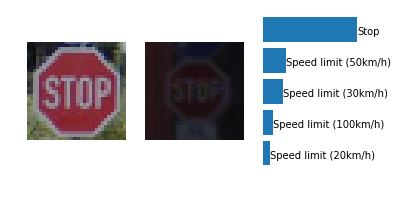
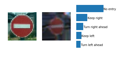
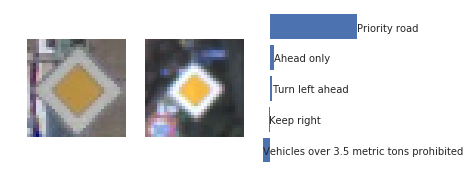
The model was able to correctly guess 6 of the 6 traffic signs, which gives an accuracy of 100%. Nice!
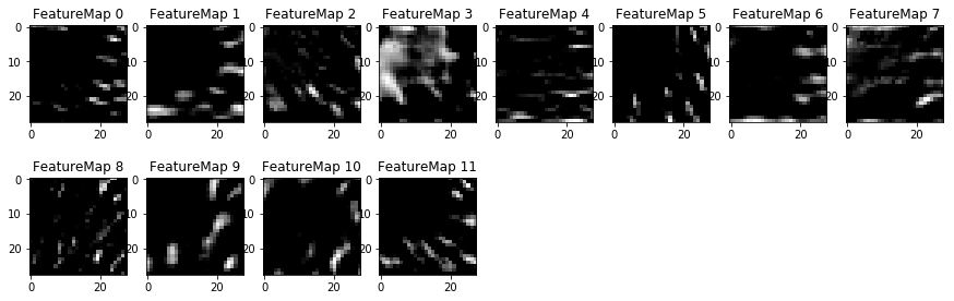
Visualize the Neural Network’s State with Test Images
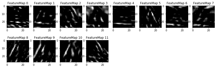
We can understand what the weights of a neural network look like better by plotting their feature maps. After successfully training your neural network you can see what it’s feature maps look like by plotting the output of the network’s weight layers in response to a test stimuli image. From these plotted feature maps, it’s possible to see what characteristics of an image the network finds interesting. For a sign, maybe the inner network feature maps react with high activation to the sign’s boundary outline or the contrast in the sign’s painted symbol.
Here the output of the first convolution layer:
Here the output of the second convolution layer:
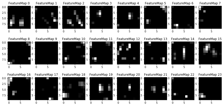
We can notice that the CNN learned to detect useful features on its own. We can see in the first picture some edges of the sign for example.
Now another example using a test picture with no sign on it:

In this case the CNN does not recognize any useful features. The activations of the first feature map appear to contain mostly noise:
Final considerations
Premise:
Only CPU was used to train the network. I had to use only the CPU of my laptop because I didn’t have any good GPU at my disposal. I choose to not use any online service like AWS or FloydHub, mostly because I was waiting for the arrival of the GTX 1080. Unfortunately, it did not arrive in time for this project. This required me to use a small network and to keep the number of epochs around 20.
Some possible improvements:
- I would use Keras to define the network and its function ImageDataGenerator to generate augmented samples on the fly. Using more data could improve the performance of the model. In my case, I have generated an augmented dataset once, saved it on the disk and used it every time to train. It would be useful to generate randomly the dataset each time before the training.
- The confusion matrix gives us suggestions to improve the model (see section
Confusion matrix). There are some classes with low precision or recall. It would be useful to try to add more data for these classes. For example, I would generate new samples for the class 19 (Dangerous curve to the left) since it has only 180 samples and the model. - The accuracy for the training set is 0.975. This means that the model is probably underfitting a little bit. I tried to make a deeper network (adding more layers) and increasing the number of filters but it was too slow to train it using the CPU only.
- The model worked well with new images taken with my camera (100% of accuracy). It would be useful to test the model by using more complicated examples.
Leave a Comment